Data Format

GF4 accepts text files with whitespace-separated columns, one data point per row. It also accepts comma-separated columns (CSV files); these are converted internally to TAB-separated columns. If the input file is a CSV file, GF4 tries to identify the column headers by looking at the row just before the first data row.

If there is only one column, GF4 inserts an imputed first column with values being consecutive integers beginning with 1. The “first” column becomes the “x”, or horizontal, axis. If there are more than two columns, a dialog is displayed so the user can choose the two desired columns. The number of columns is derived based on the first non-comment, non-blank line whose first field is a legal floating point number.

Data fields must be numeric. GF4 cannot make use of non-numeric data. Data fields are converted to floating point numbers. Date fields are not understood nor displayed. Date columns should be converted to serial numbers, such as months or years, beginning with the beginning epoch. The conversion should be done outside of GF4. Alternatively, a leading data column could be deleted. Once GF4 has loaded the data, its horizontal axis can be changed to reflect the starting point and increment by using the NewX command button.

Here is an example data file:

# A comment line
; Another comment line.  Also, blank lines are ignored.
# x  y
1  1
2  4
3  9
# etc

Data points do not need to be equally spaced on the x axis.

There are specially formatted (optional) comments to specify a title, axis labels, and a break between data sets:

;; FIGURELABEL: The Title
;; XLABEL: The x axis label
;; YLABEL: the y axis label
1    3.0
2    4.0
3    6.0
4    7.0
;; ENDDATASET

The special comment key words are case sensitive. If there is more than one dataset, the second one goes into the Y position in the stack, and so on up to the stack depth. Beyond that additional data sets are ignored.

Invalid or Missing Data

GF4 has no provision for handling invalid or missing data, except that a line in the data file that fails the attempt to convert its fields into floating point numbers will be ignored.

Editing and Censoring of Data Points

The only way that individual data points can be modified within GF4 is to copy the dataset to the system clipboard and then paste it into the Load From Dialog edit pane. In the edit pane, individual rows can be corrected or commented out.

The Waveform Stack

The waveform stack is the primary organizing concept of GF4. Modeled after the stack in Hewlett-Packard RPN calculators, the stack is an array with positions that can hold data elements. Conceptually, the stack is arranged as a vertical column with a “bottom” and a “top”. Items on the stack can be “pushed” upwards, “dropped” downwards, “rotated” and “swapped”. These operations are illustrated in the next section.

All operations that change data operate on the data in the stack bottom (the X position). All operations between two datasets, such as addition and correlation, use the X and Y positions (Y is the next position up from X 1). the result of these operations only change data in the X position. The data in Y remains unchanged.

The state of the stack can be viewed by using the Help/ Show Stack menu item in the main window. This opens a small window that shows the name of the dataset currently in each stack position. It is helpful to keep this window open while one gains experience with GF4. The image below depicts the stack viewer window:

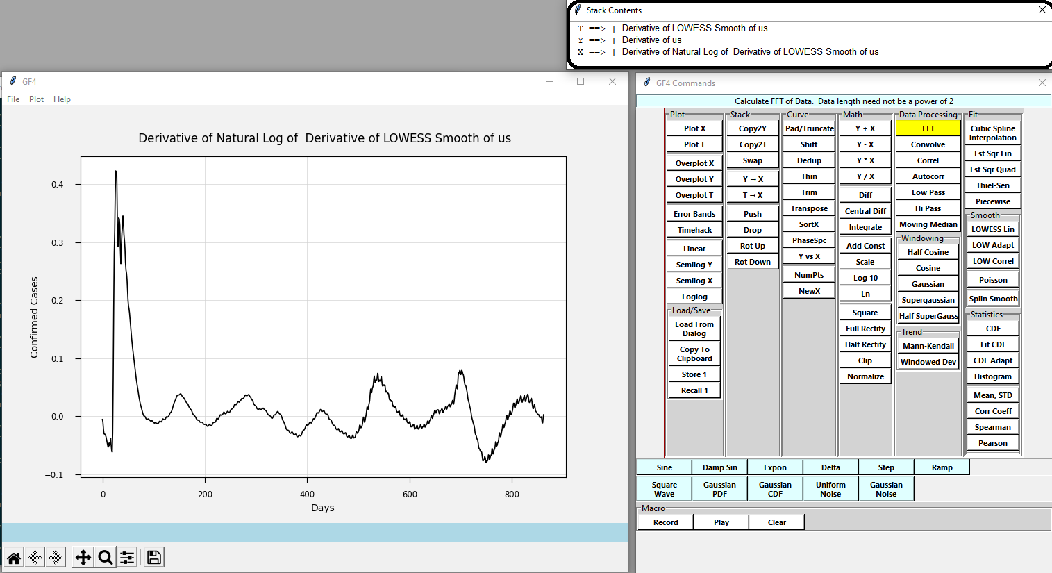
The most common stack operations in practice are “Swap” and direct access. The T position is often used as a temporary data cache.

1

For historical reasons, the Y stack position is also called the Buffer and the X position is also called Main.

Stack Operations

The stack can be “pushed”, causing the existing elements to be moved one slot “higher”:

Stack populated with data elements A, B, and C

|   A   |   <-- "T": stack top
|   B   |   <-- "Y"
|   C   |   <-- "X": stack bottom

"Pushing" stack duplicates "X" element (top element is lost)

|   B   |   <-- "T": stack top
|   C   |   <-- "Y"
|   C   |   <-- "X": stack bottom

“Dropping” the stack moves elements one slot lower:

Stack populated with data elements A, B, and C

|   A   |   <-- "T": stack top
|   B   |   <-- "Y"
|   C   |   <-- "X": stack bottom

"Dropping" stack duplicates "T" element (bottom element is lost)

|   A   |   <-- "T": stack top
|   A   |   <-- "Y"
|   B   |   <-- "X": stack bottom

The stack can also be cyclically rotated up or down:

Stack populated with data elements A, B, and C

|   A   |   <-- "T": stack top
|   B   |   <-- "Y"
|   C   |   <-- "X": stack bottom

Rotated "up" (T -> X, X -> Y, Y -> T)

|   B   |   <-- "T": stack top
|   C   |   <-- "Y"
|   A   |   <-- "X": stack bottom

Stack populated with data elements A, B, and C

|   A   |   <-- "T": stack top
|   B   |   <-- "Y"
|   C   |   <-- "X": stack bottom

Rotated "down" (T -> Y, Y -> X, X -> T)

|   C   |   <-- "T": stack top
|   A   |   <-- "Y"
|   B   |   <-- "X": stack bottom

“Swap” exchanges the X and Y data elements:

Stack populated with data elements A, B, and C

|   A   |   <-- "T": stack top
|   B   |   <-- "Y"
|   C   |   <-- "X": stack bottom

Stack after a "Swap"

|   A   |   <-- "T": stack top
|   C   |   <-- "Y"
|   B   |   <-- "X": stack bottom

Direct Access

The data element in X, the stack bottom, can be copied to the Y and T positions. The Y and T data elements can be copied to the X position. All the stack operations are carried out by clicking buttons in the auxiliary command window.

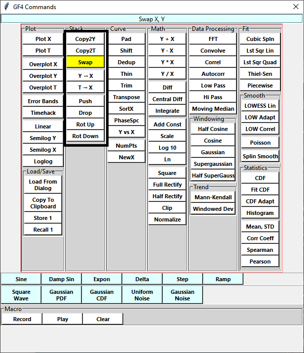
Non-Stack Storage

In addition to the stack, there are several other data storage locations:

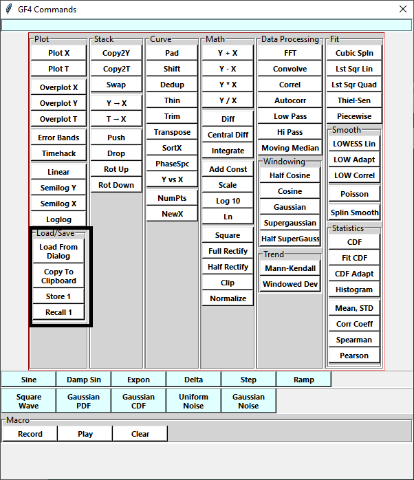
1. A single slot accessed by the Store 1* and Recall 1 buttons. These store from and retrieve to the X position.

2. The system clipboard, accessed by the Copy To Clipboard and Load From Dialog buttons. The latter opens an editing window into which the clipboard can be copied.

These buttons are marked in the image below:

Loading And Saving Data

All data is saved from and loaded to the X stack position. This will overwrite the previous contents. If you want to keep the previous data set, push or copy it to one of the other positions. Most often, the Y position is used for this.

The data format is described in Data Format. Data is saved in TAB-separated format (even if it was originally in CSV format) and includes the special comments that will recreate the title and axis labels. Error bars are not saved.

Data can be saved to a file (using the File/Save menu item) or copied to the system clipboard (using the Copy To Clipboard button). A data file can be read using the File/Open menu item. Data, including CSV-format data, can also be loaded into the X position from the system clipboard using the Load From Dialog button. Note that this dialog’s entry panel is a basic text editor, so the data from the clipboard can be edited before it is processed.

Saving Graphs

The visible graph can be saved as an image file, such as a .png file. The standard MatPlotLib toolbar that GF4 displays near the bottom of the main window includes a button with an icon of a floppy disk. Clicking this button opens the image save dialog. There is no provision for loading an image into GF4, since it would not contain the numeric data in a form that GF4 could use.

Plotting Curves

Plotting commands are grouped together in the Command Window:

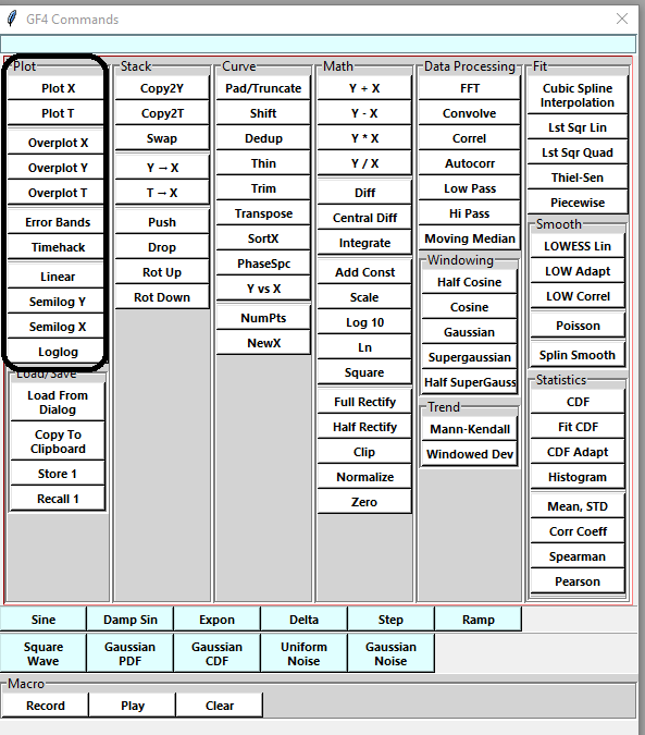
Figure BA-1. Plotting Buttons in the Command Window.

These same commands are also available in the Plot menu in the main GF4 window. This menu is also the only place where the graph properties can be changed. These properties include line width and color, whether to use symbols instead of lines and if so, which symbol shape to use.

Data in any of the three stack positions X, Y, and T can be overplotted; Only X and T can be plotted. These terms mean the following:

• Plot – create a new graph at displays the specified data set;

• Overplot – plot a dataset on top of an existing graph. The axes may rescale if the new data would overflow the previous bounds of the graph.

Overplotting is essential to getting the most out of GF4, since it provides a way to compare several data sets, or several ways of processing the same data.

Default Plotting Settings

When GF4 starts up, it sets the following values for the plotting attributes:

Default Plot Settings

Stack Position	Color	Line Thickness	Line/Symbol
X	black	medium	line
Y	cyan	medium	line
T	black	thin	line

These values are chosen to make it easy to distinguish between the data sets when overplotted. The lighter color of the medium cyan line of the Y dataset is easy to distinguish from the medium weight black of the X dataset, while the lighter appearance of the cyan does not distract much from the heavier weight black line. The thin black line of the T dataset is easy to distinguish from the other two.

When GF4 starts up, no stack position has data, so there is nothing to plot. When the first data set is read, it is automatically plotted. When other datasets are read, GF4 notices that there is already data in the X stack position, and it does not plot the new data. This allows the user to keep reading data files and overplotting them - possibly in different colors - without destroying an existing graph. This can be a very useful capability.

Changing Colors, Symbols, and Line Styles

Curve plotting options can be changed for plotting/overplotting data in the X and Y stack positions. The line and color styles of the T* position cannot be changed. In practice, this is rarely a problem. Technically there would be no problem in providing for changes in the T appearance, but up until now it has seemed not to be worth the extra complexity for the user. Changing these properties using menus is a little tedious, but adding buttons to the command window would be bad for its readability and usability.

Figure BA-2 depicts the Plot menu items that can change the appearance of X and Y data:

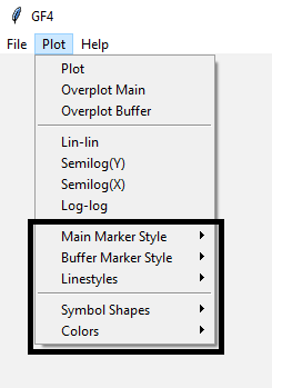
Figure BA-2. Plot Menu Items For Changing Plotting Options.

These menu items are reasonably self-explanatory. For example, Figure BA-3 shows one of the menus expanded:

Figure BA-3. Selecting the “Buffer” (Y) Plotting Style 2.

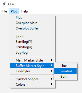
2

As mentioned in The Waveform Stack, the Y position is also called the Buffer, and the X position may be called Main.

Help For Commands

For the commands that have buttons in the Command Window, hovering the mouse over the button causes a brief summary to display in the band at the top of the Command window. Right-clicking on a button displays a more detailed explanation in the system browser.

If an extended help message does not exist for the button, this will be announced in the announcement bar at the bottom of the main window.